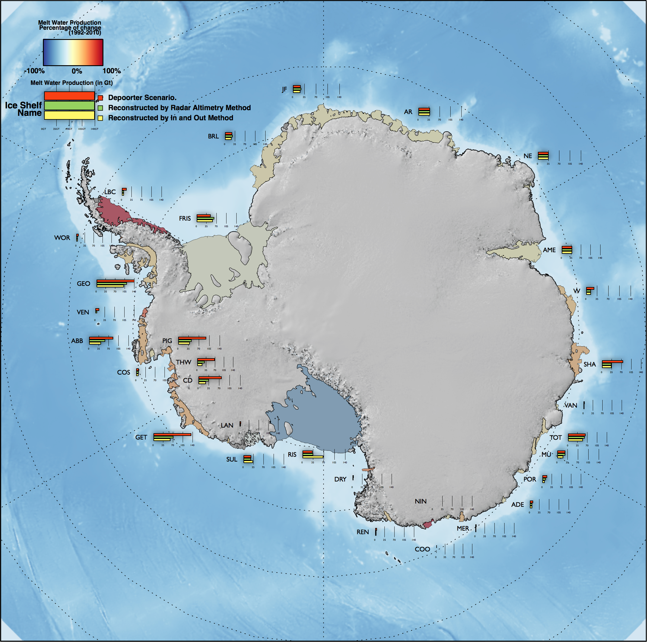
Plotting continents... shapefiles and tif images with Cartopy

Posted by Nacho on January 20, 2016 7 minute read ∼ Tagged with : Nemo • Cartopy • Python ∼ Filed in : Nemo • Python

Plotting Antarctica with Cartopy and GDAL libraries

I will explain the way I plot the Antarctic continent including extra-features from tiff files like the mountains relief and/or the ocean bathymetry. All those files (shapefiles and tiff images) are extracted from the Antarctic Digital DataBase (http://http://www.add.scar.org/home/add7), containing a long list of digital data open to be downloaded by any user. The method I will explain can be applied to other parts of the world with different data or projections, you just need to get the source .shp file corresponding to your region of interest, and tiff images (for example photos from satellites). This is just an example to illustrate the flexibility of those tools, the GDAL and ShapeReader from Cartopy.

First of all he have to create the shapefile reader. This is the python object for reading .shp, which includes various geometries (lines, surfaces or points).

import cartopy.io.shapereader as shpreader
#cst10_polygon.shp is downloaded http://www.add.scar.org/home/add7 from 
fname= '/Users/imerino/Documents/These/python/Data/cst10_polygon.shp' 
reader = shpreader.Reader(fname)

In this example I want to draw differently the land, the calving front, the grounding line and the ice shelves. Using the reader object we can have access to all the geometries and their properties. We can easily loop over the geometries and individually plot them depending of their properties.

    for line in reader.records():
        if line.attributes['cst10srf']=='iceshelf': #It's an iceshelf element
            ax.add_geometries(line.geometry, South() ,facecolor='grey' 
                , edgecolor='black',linewidth=0.2, zorder=10) 
        if line.attributes['cst10srf']!='iceshelf': #It's not an iceshelf element
            ax.add_geometries(line.geometry, South(),facecolor='none'
                , edgecolor='black',linewidth=0.5, zorder=5)

Here, the elements of my file cst10_polygon.shp have an attribute called cst10srf which tells me wether the element is part of an ice shelf or not. Ice shelf elements are plotted in grey with a black bordure (width of 0.2). Land elements will have just a thicker bordure. Axes object `ax` needs to be previously created by defining their projection and extent, The method `add_geometries()` needs the projection of the data to be plotted. According to the information given by Antarctic Digital Database, we can create my own projection `South()` extending the Projection class from Cartopy:

class South(cartopy.crs.Projection):
    def __init__(self):

        # see: http://www.spatialreference.org/ref/epsg/3408/
        proj4_params = {'proj': 'stere',
            'lat_0': -90.,
            'lon_0': 0,
            'lat_ts':-71,
            'x_0': 0,
            'y_0': 0,
            #'a': 6371228,
            #'b': 6371228,
            'a':6378137,
            'b':298.2572235630016,
            'units': 'm',
            'datum':'WGS84',
            #'ellipse':'WGS84',
            'no_defs': ''}

        super(South, self).__init__(proj4_params)

    @property
    def boundary(self):
        coords = ((self.x_limits[0], self.y_limits[0]),(self.x_limits[1], self.y_limits[0]),
                  (self.x_limits[1], self.y_limits[1]),(self.x_limits[0], self.y_limits[1]),
                  (self.x_limits[0], self.y_limits[0]))

        return cartopy.crs.sgeom.Polygon(coords).exterior

    @property
    def threshold(self):
        return 1e5

    @property
    def x_limits(self):
        return (-12400000,12400000)

    @property
    def y_limits(self):
        return (-12400000, 12400000)

I have now all my geometries plotted in my ax matplotlib axes. But we have still to draw the bathymetry and the hillshade. We will use Gdal for that:


    import gdal

    gtif = gdal.Open('/Users/imerino/Documents/These/python/Data/timmermann_bathy.tif')

    arr = gtif.ReadAsArray()   #Values
    trans = gtif.GetGeoTransform()  #Defining bounds
    extent = (trans[0], trans[0] + gtif.RasterXSize*trans[1],
            trans[3] + gtif.RasterYSize*trans[5], trans[3])

    #Open GeoTIFF hillshade file from (http://www.add.scar.org/home/add6)
    gtif2 = gdal.Open('/Users/imerino/Documents/These/python/Data/hillshade.tif')

    arr2 = gtif2.ReadAsArray()  #Values
    trans2 = gtif2.GetGeoTransform() #Defining bounds
    extent2 = (trans2[0], trans2[0] + gtif2.RasterXSize*trans2[1],
            trans2[3] + gtif2.RasterYSize*trans2[5], trans2[3])

    arr[:,:]=-arr[:,:]*(arr>-1e20)
    arr2[:,:]=-arr2[:,:]*(arr2>-1e20)

Here both .tif files (image with geospatial coordinates) are opened and readed. the extent for both images will be used later for plotting with imshow. NaN values are masked to 0.

Before finishing, there is something to do with the hillshade data. My hillshade file is defined also out of the Antarctic continent, I don't want the hillshade image to be over the bathymetry image in the ocean regions, and I don't want the bathymetry to be over the hillshade in land regions. To solve that we can set the transparency to 0 for the first 10 levels of the hillshade by doing the following:

    c = mcolors.ColorConverter().to_rgb

    color1 = colorConverter.to_rgba('white')
    color2 = colorConverter.to_rgba('black')

    # make the colormaps
    cmap2 = mpl.colors.LinearSegmentedColormap.from_list('my_cmap2',[color1,color2],256)
    cmap2._init() # create the _lut array, with rgba values

    # create your alpha array and fill the colormap with them.
    # here it is progressive, but you can create whathever you want
    cmap2._lut[0:10,-1] = 0.0  #We made transparent de 10 first levels of hillshade, 
    cmap2._lut[10:cmap2.N+3-1,-1] = 0.99

Basically, a color bar from white to black is created from the hillshade data, and the transparency is set to zero for the first 10 altitude levels (so the ocean and coastal regions in the image wont be visible). This color bar will be used during the drawing of the hillshade as we will see.

    cax=ax.imshow(arr[:,:].transpose(),extent=extent,transform=South2(),cmap='Blues',
        alpha=0.7)
    ax.imshow(arr2[:,:].transpose(),extent=extent2,transform=South3(),cmap=cmap2
        ,zorder=2)
    #cbar = plt.colorbar(cax)

Finally, both images are plotted by using imshow function from matplotlib. The projection for both plots are created in the same way than South() (see above).

Here an example of a figure having all those features decribed:

alt text

Plotting Antarctica with Cartopy and GDAL libraries

First of all he have to create the shapefile reader. This is the python object for reading .shp, which includes various geometries (lines, surfaces or points).

In this example I want to draw differently the land, the calving front, the grounding line and the ice shelves. Using the reader object we can have access to all the geometries and their properties. We can easily loop over the geometries and individually plot them depending of their properties.

I have now all my geometries plotted in my ax matplotlib axes. But we have still to draw the bathymetry and the hillshade. We will use Gdal for that:

Here both .tif files (image with geospatial coordinates) are opened and readed. the extent for both images will be used later for plotting with imshow. NaN values are masked to 0.

Basically, a color bar from white to black is created from the hillshade data, and the transparency is set to zero for the first 10 altitude levels (so the ocean and coastal regions in the image wont be visible). This color bar will be used during the drawing of the hillshade as we will see.

Finally, both images are plotted by using imshow function from matplotlib. The projection for both plots are created in the same way than South() (see above).

Here an example of a figure having all those features decribed:

Share this post